Scripts
The enclosed script along with the config file serves the same purpose as the Jupyter Notebook presented in the prior section, though it allows for more automation and possible batch computations.
To run the script, just do:
python eh_shell.py --config eh_shell.yaml
Prior to delving into the code its worth commenting on the .yaml to .py translation. Initially, the .py script load and parse the .yaml configuration script by:
cfg = get_config_file(parse_arguments())
As mentioned earlier, .yaml files are interpreted as Python dictionary. Please bear in mind that the configuration script is totally optional. If you do not wish to utilise it, just key-in the desired values/strings/parameters where appropriate. In order to intuitively catch how this configuration file works, let’s analyse a few examples.
Nested Directives. Please note that one can nest – theoretically – an indefinite number of directive levels. Nonetheless, the example uses only double nested directive to keep the configuration file manageable and easy to read. For instance, consider:
logger_manager(level=cfg["logger"]["level"])
this looks for the key logger and for the sub-key level in the .yaml script, which correspond to the following lines:
logger:
    level: WARNING
Without the configuration file:
logger_manager(level="WARNING") # for instance
Unnested Directives. Consider for instance:
sd = SyntheticDataset(name=cf["name"])
this looks for the key name directly:
name: aString
Without the configuration file:
sd = SyntheticDataset(name="aString")
Overview of the Script
The script generates a regular training grid upon an El Haddad curve having \(\Delta K_{th,lc} = 8\), \(\Delta\sigma_w = {700}\), \(Y=0.9\) (this values are arbitrarily taken). The script shall return the parameters of the curve that generated the dataset. In this instance, we should not prescribe priors, nor use a normalised log-likelihood.
The figures below display the results obtained, which are consistent with the hypothesised curve.
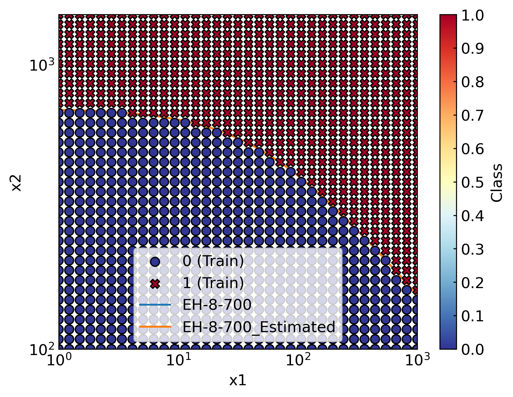
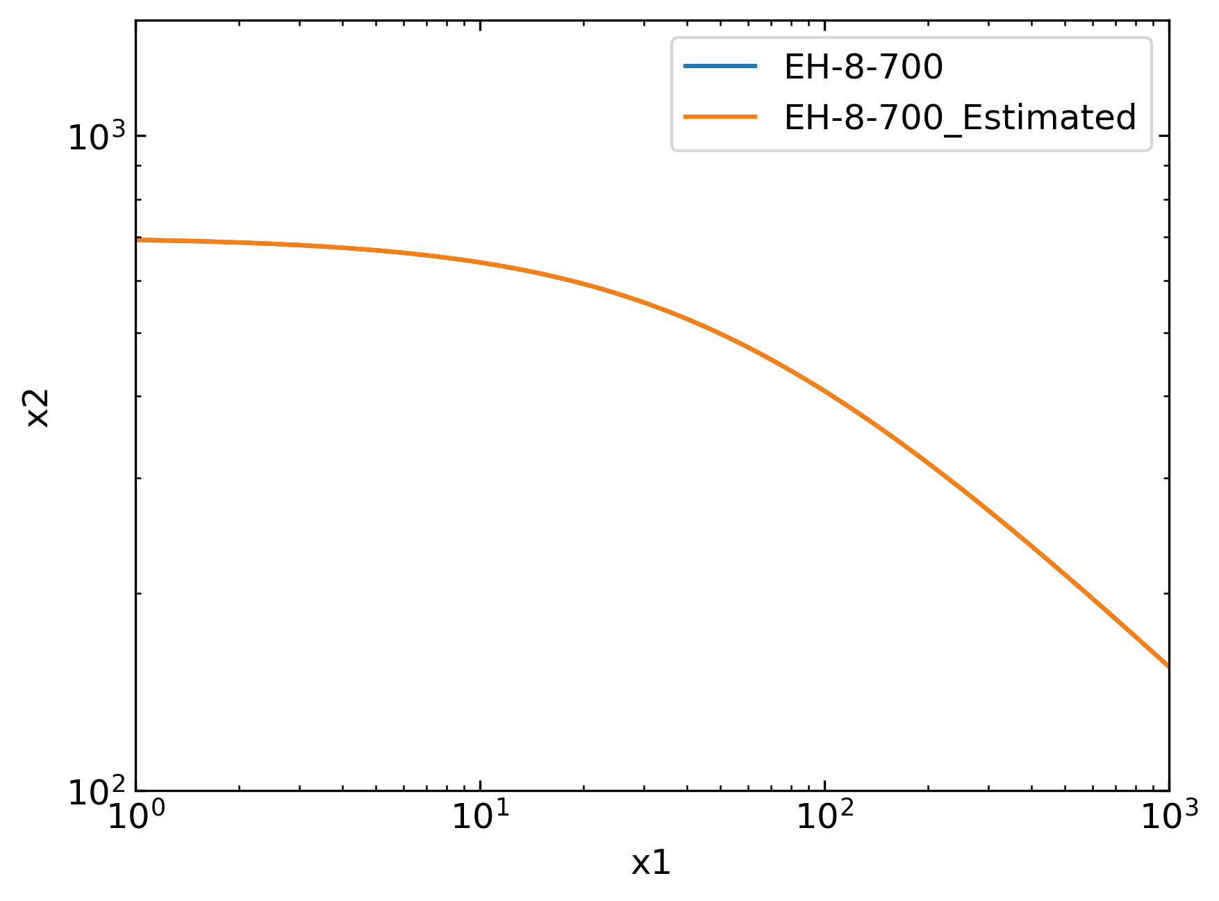
Please note that labels are generic as the processed dataset is not instantiated from ElHaddadDataset. Importantly, we did not compute the predictive posterior as the estimation process just run Maximum Likelihood Estimation. Hence, the posterior is not envisaged in this framework.
Python Script
#%% Import required modules and configure common parameters
from sys import path as syspath
from os import path as ospath
syspath.append(ospath.join(ospath.expanduser("~"),
                           '/home/ale/Desktop/b-fade/src'))

# Erase the line above if you installed the package.

import numpy as np
import sklearn.metrics

from bfade.elhaddad import ElHaddadCurve, ElHaddadBayes
from bfade.dataset import SyntheticDataset
from bfade.viewers import BayesViewer, PreProViewer
from bfade.util import parse_arguments, get_config_file, config_matplotlib, logger_manager

cf = get_config_file(parse_arguments("./eh_shell.yaml"))

logger_manager(level=cf["logger"]["level"])

config_matplotlib(font_size=cf["matplotlib"]["font_size"],
                  font_family=cf["matplotlib"]["font_family"],
                  use_latex=cf["matplotlib"]["use_latex"],
                  interactive=cf["matplotlib"]["interactive"])

# Istantiate the ground truth EH curve
eh = ElHaddadCurve(metrics=getattr(np, cf["curve"]["metrics"]),
                   dk_th=cf["curve"]["dk_th"],
                   ds_w=cf["curve"]["ds_w"],
                   Y=cf["curve"]["Y"],
                   name=cf["name"])
eh.config(save=cf["export"]["save"], folder=cf["export"]["folder"])
eh.inspect(np.linspace(cf["inspect_eh"]["start"],
                       cf["inspect_eh"]["stop"],
                       cf["inspect_eh"]["step"]),
                       scale=cf["inspect_eh"]["scale"])

# Generate training dataset
sd = SyntheticDataset(name=cf["name"])
sd.config(save=cf["export"]["save"], folder=cf["export"]["folder"])
sd.make_grid(cf["train"]["x1"], cf["train"]["x2"],
             cf["train"]["n1"], cf["train"]["n2"],
             spacing=cf["train"]["spacing"])
sd.make_classes(eh)
sd.inspect(cf["train"]["x1"], cf["train"]["x2"], scale=cf["train"]["spacing"],
           curve=eh, x=np.linspace(cf["inspect_eh"]["start"],
                                   cf["inspect_eh"]["stop"],
                                   cf["inspect_eh"]["step"]))

# Initialise Bayesian Infrastructure
bay = ElHaddadBayes("dk_th", "ds_w", Y=cf["curve"]["Y"], name=cf["name"])
bay.load_log_likelihood(getattr(sklearn.metrics, cf["log_likelihood"]["function"]),
                        normalize=cf["log_likelihood"]["normalize"])

# Inspect likelihood (which coincides in this case) before MAP
v = BayesViewer("dk_th", cf["inspect_bayes"]["b1"], cf["inspect_bayes"]["n1"],
                "ds_w" , cf["inspect_bayes"]["b2"], cf["inspect_bayes"]["n2"],
                name=cf["name"])
v.config(save=cf["export"]["save"], folder=cf["export"]["folder"])
# v.contour("log_likelihood", bay, sd)

# Run MAP
bay.MAP(sd, cf["map_guess"])

# Get Optimal EH curve
opt = ElHaddadCurve(dk_th=bay.theta_hat[0], ds_w=bay.theta_hat[1], Y=cf["curve"]["Y"],
                    name=cf["name"] + "_Estimated")
opt.config(save=cf["export"]["save"], folder=cf["export"]["folder"])
opt.inspect(np.linspace(cf["inspect_eh"]["start"],
                        cf["inspect_eh"]["stop"],
                        cf["inspect_eh"]["step"]),
                        scale=cf["inspect_eh"]["scale"])

# View results
p = PreProViewer(cf["train"]["x1"], cf["train"]["x2"],
                 cf["inspect_eh"]["step"], cf["inspect_eh"]["scale"],
                 name=cf["name"])
p.config(save=cf["export"]["save"], folder=cf["export"]["folder"])
p.view(train_data=sd, curve=[eh, opt])
p.view(curve=[eh, opt])

print(bay.theta_hat)
Yaml Config Script
name: EH-8-700

logger:
  level: DEBUG

matplotlib:
  font_size: 12
  font_family: sans-serif
  use_latex: False
  interactive: True

export:
  save: True
  folder: ./

inspect_eh:
  start: 1
  stop: 1000
  step: 2000
  scale: log

inspect_bayes:
  b1: [5,10]
  b2: [500, 900]
  n1: 20
  n2: 20

train:
  x1: [1,1000]
  x2: [100, 1500]
  n1: 35
  n2: 35
  spacing: log

curve:
  dk_th: 8
  ds_w: 700
  Y: 0.9
  metrics: log10

log_likelihood:
  function: log_loss
  normalize: False #!!!

map_guess: [6, 500]